Example 5: Apply an SSE method for wave spectrum estimation from vessel responses

1. Introduction

In this example, it is shown how ship motions can be analyzed with the NetSSE package to estimate important characteristics of the encountered sea state.

The following modules and packages are imported:

import matplotlib.pyplot as plt
import numpy as np
from scipy.signal import csd

from netsse.analys.sawb import genspecres
from netsse.dataset import load_example_data
from netsse.tools.viz import fig_settings

===============================
Registration Request for NetSSE
To help us improve and better understand our user community, we kindly ask all users to register to use NetSSE. Registration is free.
If you have not already registered, please do so here:
https://forms.office.com/Pages/ResponsePage.aspx?id=I_FR8s7JjkSSdzS7KFkR2Xd1K-8FtOJFrL9QLVM8cJZUQ1hBS0VTN1E0OVU4QThTOTQ1WDA0TFg4Si4u
===============================

As can be seen in the above import, this example illustrates the use of the following NetSSE functions:

• fig_settings(...),

• load_example_data(...),

• genspecres(...) from the analys.sawb module

Define default settings

Those settings are used for the visual appearance of figures generated in this Python example.

fig_path, figcolors, props = fig_settings(font="serif", dpi=100, usetex=True)

Import the measurement data

The input data to this example are the time series of vessel motions measured on-board. The time series are synchronized and sampled at 2 Hz.

The time series are read from a .csv file in Pandas.

df_motion = load_example_data("response_time_series.csv", index_col=0)
print("Table 1: Measurements of vessel motions.")
df_motion

Table 1: Measurements of vessel motions.

	time	heave	pitch	vbm
0	0.0	-0.053065	0.117952	86.069354
1	0.5	-0.042642	0.119615	89.683259
2	1.0	-0.027279	0.106653	87.766492
3	1.5	-0.008232	0.082540	80.844487
4	2.0	0.012907	0.051804	69.527379
...	...	...	...	...
2395	1197.5	0.054573	0.052047	92.396714
2396	1198.0	0.066896	0.066212	5.765010
2397	1198.5	0.071972	0.078243	-83.249914
2398	1199.0	0.069147	0.086857	-164.981687
2399	1199.5	0.058790	0.090813	-230.495060

2400 rows × 4 columns

2. Analysis of the vessel motions

The vessel motions have been measured for a twenty-minute segment duration. During this segment, the vessel’s heading is nearly constant to 180 deg, which means that the vessel is navigating towards South.

The response measurement data is provided here.

We now analyse the heave, pitch, and vertical bending moment (VBM) motions of the vessel during the segment.

time = df_motion["time"].values
heave = df_motion["heave"].values
pitch = df_motion["pitch"].values
vbm = df_motion["vbm"].values
units = ["m", "deg", "kNm"]

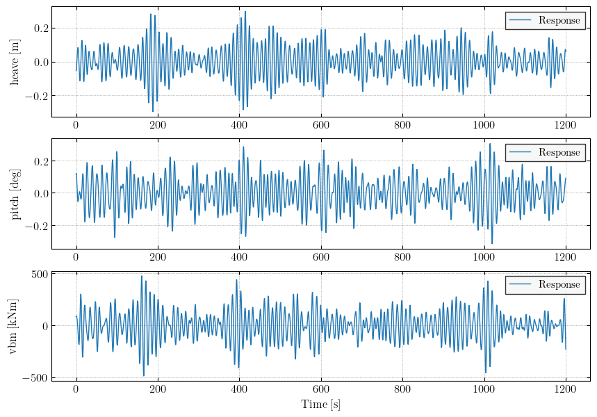
We plot the time series of the response measurements.

fig, ax = plt.subplots(3, 1, figsize=(10, 7))
for i_plot in range(3):
    ax[i_plot].plot(time, df_motion.iloc[:, i_plot + 1], label="Response")
    ax[i_plot].set_ylabel(df_motion.columns[i_plot + 1] + " [" + units[i_plot] + "]")
    ax[i_plot].grid()
    ax[i_plot].legend()
ax[-1].set_xlabel("Time [s]")
# fig.tight_layout()
print('Fig. 1: Response measurement time series.')
plt.show()

Fig. 1: Response measurement time series.

Now, we compute the response spectra of the heave, pitch, and VBM signals, using the Welch algorithm.

nperseg = 2**9  # Number of samples per segment for spectral estimation
fs = 1 / np.mean(np.diff(time))  # Sampling frequency of the measurements [Hz]

# Compute the auto-spectral densities of the responses using Welch's method:
freq, Sr33 = csd(
    heave,
    heave,
    fs=fs,
    window="parzen",
    nperseg=nperseg,
)
freq, Sr55 = csd(
    pitch,
    pitch,
    fs=fs,
    window="parzen",
    nperseg=nperseg,
)
_, Srvv = csd(
    vbm,
    vbm,
    fs=fs,
    window="parzen",
    nperseg=nperseg,
)

# Compute the cross-spectral density between pairs of responses:
_, Sr35 = csd(
    heave,
    pitch,
    fs=fs,
    window="parzen",
    nperseg=nperseg,
)
_, Sr3v = csd(
    heave,
    vbm,
    fs=fs,
    window="parzen",
    nperseg=nperseg,
)
_, Sr5v = csd(
    pitch,
    vbm,
    fs=fs,
    window="parzen",
    nperseg=nperseg,
)

# Truncate the spectrum to the frequency range of interest:
freq_ub = 0.25
freq_idx = freq <= freq_ub
freq = freq[freq_idx]
Sr33 = np.real(Sr33[freq_idx])
Sr55 = np.real(Sr55[freq_idx])
Srvv = np.real(Srvv[freq_idx])
Sr35 = Sr35[freq_idx]
Sr3v = Sr3v[freq_idx]
Sr5v = Sr5v[freq_idx]

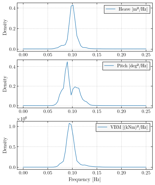
Plot the auto-spectral desnsities of the measured responses.

spectra_plot = [Sr33, Sr55, Srvv]
legend_labels = ["Heave [m²/Hz]", "Pitch [deg²/Hz]", "VBM [(kNm)²/Hz]"]
fig, ax = plt.subplots(3, 1, figsize=(5, 6), constrained_layout=True)
for i_plot in range(3):
    ax[i_plot].plot(freq, spectra_plot[i_plot], label=legend_labels[i_plot])
    ax[i_plot].set_ylabel("Density")
    ax[i_plot].legend()
    ax[i_plot].grid()
ax[-1].set_xlabel("Frequency [Hz]")
# fig.tight_layout()
print('Fig. 2: Auto-spectral densities of the responses.')
plt.show()

Fig. 2: Auto-spectral densities of the responses.

3. Analyse the vessel’s transfer functions

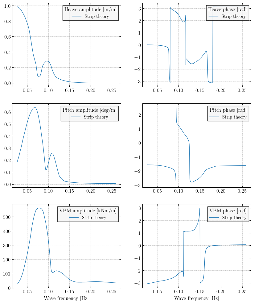
In this section, we analyse RAOs of the studied vessel, obtained via a linear strip theory solver, the so-called New Strip Method (Takagi and Ganno, 1967), in which the Lewis form approximation of ship cross-sections is adopted. For more detail, refer to Takami et al. (2026).

The amplitude and phase of the strip theory transfer functions of heave and pitch motions, as well as vertical bending moment (VBM), are provided here in a data file named "strip_theory_TRFs_full.txt".

Load the transfer functions derived by strip theory

The data file is organized as shown in Table 2.

Table 2: File structure for the strip_theory_TRFs.txt data file.

	Column 0	Column 1	Column 2	Column 3	Column 4	Column 5	Column 6	Column 7
Row 0	Frequency_1	Heading_1	Heave amp.	Heave phase	Pitch amp.	Pitch phase	VBM amp.	VBM phase
Row 1	Frequency_2	Heading_1
…	…	…	…	…	…	…	…
Row Nf-1	Frequency_Nf	Heading_1
Row Nf	Frequency_1	Heading_2
Row Nf+1	Frequency_2	Heading_2
…	…	…	…	…	…	…	…
Row 2Nf-1	Frequency_Nf	Heading_2
…	…	…	…	…	…	…	…
Row NhxNf-1	Frequency_Nf	Heading_Nh

ST_data = load_example_data("strip_theory_TRFs_full.txt", delimiter="\t")
f0_ST = np.sort(np.unique(ST_data[:, 0]))
beta_ST = np.sort(np.unique(ST_data[:, 1]))
Nf0 = len(f0_ST)
Nbeta = len(np.unique(beta_ST))

hamp_ST = ST_data[:, 2]
hphase_ST = ST_data[:, 3]
pamp_ST = ST_data[:, 4]
pphase_ST = ST_data[:, 5]
vamp_ST = ST_data[:, 6]
vphase_ST = ST_data[:, 7]

We reorganize the data in 2-D arrays, so that each column corresponds to a distinct heading.

hamp_ST = hamp_ST.reshape((Nbeta, Nf0)).T
hphase_ST = hphase_ST.reshape((Nbeta, Nf0)).T
pamp_ST = pamp_ST.reshape((Nbeta, Nf0)).T
pphase_ST = pphase_ST.reshape((Nbeta, Nf0)).T
vamp_ST = vamp_ST.reshape((Nbeta, Nf0)).T
vphase_ST = vphase_ST.reshape((Nbeta, Nf0)).T

Plot the transfer functions estimated by strip theory

The strip theory transfer functions are plotted together with the transfer functions estimated by the closed-form expressions (Jensen et al., 2004) for comparison. A heading of \(\beta = 180\) degrees is selected for plotting.

legend_titles = [
    r"Heave amplitude [m/m]",
    r"Heave phase [rad]",
    r"Pitch amplitude [deg/m]",
    r"Pitch phase [rad]",
    r"VBM amplitude [kNm/m]",
    r"VBM phase [rad]",
]
fig, ax = plt.subplots(3, 2, figsize=(10, 12))
ax[0, 0].plot(f0_ST, hamp_ST[:, -1], label=r"Strip theory")
ax[0, 1].plot(f0_ST, hphase_ST[:, -1], label=r"Strip theory")
ax[1, 0].plot(f0_ST, pamp_ST[:, -1], label=r"Strip theory")
ax[1, 1].plot(f0_ST, pphase_ST[:, -1], label=r"Strip theory")
ax[2, 0].plot(f0_ST, vamp_ST[:, -1], label=r"Strip theory")
ax[2, 1].plot(f0_ST, vphase_ST[:, -1], label=r"Strip theory")
for i in range(3):
    for j in range(2):
        ax[i, j].grid()
        ax[i, j].legend(title=legend_titles[i * 2 + j])
        ax[-1, j].set_xlabel(r"Wave frequency [Hz]")
print('Fig. 3: Strip theory response amplitude operators (RAOs) and phases for the vessel in head sea conditions.')
# fig.tight_layout()
plt.show()

Fig. 3: Strip theory response amplitude operators (RAOs) and phases for the vessel in head sea conditions.

4. Sea state estimation - Long-crested wave case

Now, we will run a simple WBA algorithm to estimate the point wave spectrum from response measurements. We assume that the sea state is long-crested.

The spectral-residual algorithm is used. This algorithm was initially proposed by Brodtkorb et al. (2018a,b & 2023) and Nielsen et al. (2018).

The first step is to prepare the input.

1. We gather the response spectra into a single array for use in the NetSSE analysis.

Rxy = np.column_stack([Sr33, Sr55, Srvv]).T

2. We interpolate the transfer functions at the frequencies of the computed response spectra, and we gather the transfer functions into a single array for use in the NetSSE analysis.

hamp_ST_interp = np.array([np.interp(freq, f0_ST, hamp_ST[:, i]) for i in range(Nbeta)])
pamp_ST_interp = np.array([np.interp(freq, f0_ST, pamp_ST[:, i]) for i in range(Nbeta)])
vamp_ST_interp = np.array([np.interp(freq, f0_ST, vamp_ST[:, i]) for i in range(Nbeta)])

Hxy = np.concatenate(
    [
        np.array(hamp_ST_interp)[np.newaxis, :, :],
        np.array(pamp_ST_interp)[np.newaxis, :, :],
        np.array(vamp_ST_interp)[np.newaxis, :, :],
    ],
    axis=0,
)

We run the spectral-residual SSE algorithm.

S_wave, beta_est, num_it = genspecres(Rxy, Hxy, freq, beta_ST, opt=None)

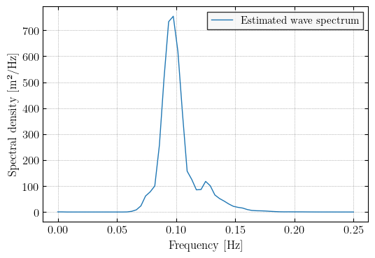
We plot the estimated wave spectrum.

fig = plt.figure(figsize=(6, 4))
plt.plot(freq, S_wave, label=r"Estimated wave spectrum")
plt.xlabel("Frequency [Hz]")
plt.ylabel(r"Spectral density [m²/Hz]")
plt.grid()
plt.legend()
print('Fig. 4: Estimated wave spectrum using the WBA method.')
plt.show()

Fig. 4: Estimated wave spectrum using the WBA method.

References

1. Brodtkorb, A.H., Nielsen, U.D., & Sørensen, A.J. (2018a). Online wave estimation using vessel motion measurements. IFAC-PapersOnLine 51(29), 244–249. https://doi.org/10.1016/j.ifacol.2018.09.510

2. Brodtkorb, A.H., Nielsen, U.D., & Sørensen, A.J. (2018b). Sea state estimation using vessel response in dynamic positioning. Applied Ocean Research 70, 76–86. https://doi.org/10.1016/j.apor.2017.09.005

3. Nielsen, U.D., Brodtkorb, A.H., & Sørensen, A.J. (2018). A brute-force spectral approach for wave estimation using measured vessel motions. Marine Structures 60, 101–121. https://doi.org/10.1016/j.marstruc.2018.03.011

4. Brodtkorb, A.H., & Nielsen, U.D. (2023). Automatic sea state estimation with online trust measure based on ship response measurements. Control Engineering Practice 130. https://doi.org/10.1016/j.conengprac.2022.105375