Example 1: Characterize a sea state from sea surface elevation time series

1. Introduction

In this first example, it is shown how NetSSE can be used to analyse measurements at the sea surface. In particular, measurements of the water elevation by three wave probes around a single-point location are exploited to derive a wave spectrum and extract sea state parameters.

We would like to assess whether the three probes are experiencing the same sea state.

Import relevant packages

The following modules and packages are imported:

import matplotlib.pyplot as plt
import numpy as np
import pandas as pd

from netsse.analys.spec import spec1d_to_params
from netsse.dataset import load_example_data
from netsse.tools.viz import fig_settings

===============================
Registration Request for NetSSE
To help us improve and better understand our user community, we kindly ask all users to register to use NetSSE. Registration is free.
If you have not already registered, please do so here:
https://forms.office.com/Pages/ResponsePage.aspx?id=I_FR8s7JjkSSdzS7KFkR2Xd1K-8FtOJFrL9QLVM8cJZUQ1hBS0VTN1E0OVU4QThTOTQ1WDA0TFg4Si4u
===============================

Matplotlib is building the font cache; this may take a moment.

As can be seen in the above import, this example illustrates the use of the following NetSSE functions:

• fig_settings(...),

• load_example_data(...),

• spec1d_to_params(...).

• …

Define default settings

Those settings are used for the visual appearance of figures generated in this Python example.

fig_path, figcolors, props = fig_settings(font="serif", dpi=100, usetex=True)

Import the measurement data

The input data to this example are the time series of sea surface elevation (in meters) measured by the three wave probes (WP1, WP2, and WP3), which have been deployed around the same location. The time series are synchronized and sampled at 20 Hz.

The time series are read from a .csv file in Pandas. The file is named "example_WP_meas.csv" located here.

df_WP = load_example_data("example_WP_meas.csv", index_col=0)
print("Table 1: Surface measurements of wave parameters at a given location.")
df_WP

Table 1: Surface measurements of wave parameters at a given location.

	time	WP1	WP2	WP3
0	0.00	-0.054108	0.108216	-0.054108
1	0.05	-0.077697	0.155393	-0.077697
2	0.10	-0.101172	0.202345	-0.101172
3	0.15	-0.124362	0.248723	-0.124362
4	0.20	-0.147087	0.294173	-0.147087
...	...	...	...	...
447205	22360.25	-0.018386	0.036773	-0.018386
447206	22360.30	-0.016299	0.032598	-0.016299
447207	22360.35	-0.014064	0.028128	-0.014064
447208	22360.40	-0.011657	0.023313	-0.011657
447209	22360.45	-0.009051	0.018102	-0.009051

447210 rows × 4 columns

2. Analyse the time series data

These time series are quite long (around 22360 s, that is approximately 6.2 hours). We will therefore limit our analysis to the first hour of the data.

time_lb = 0  # Lower bound of time segment to be analyzed
time_ub = 3600  # Upper bound
df_WP_seg = df_WP[(df_WP["time"] >= time_lb) & (df_WP["time"] < time_ub)]
print("Table 2: Extracted time segment of surface measurements for analysis.")
df_WP_seg

Table 2: Extracted time segment of surface measurements for analysis.

	time	WP1	WP2	WP3
0	0.00	-0.054108	0.108216	-0.054108
1	0.05	-0.077697	0.155393	-0.077697
2	0.10	-0.101172	0.202345	-0.101172
3	0.15	-0.124362	0.248723	-0.124362
4	0.20	-0.147087	0.294173	-0.147087
...	...	...	...	...
71995	3599.75	-0.105144	0.210289	-0.105144
71996	3599.80	-0.082366	0.164733	-0.082366
71997	3599.85	-0.059133	0.118266	-0.059133
71998	3599.90	-0.035533	0.071067	-0.035533
71999	3599.95	-0.011661	0.023322	-0.011661

72000 rows × 4 columns

Plot the time series segment for different wave probes

We would like to visually inspect the time series, to check for any major issue with the data. The three time series are plotted in three different panels (subplots) using the Matplotlib package.

colors = [figcolors["blue"], figcolors["green"], figcolors["orange"]]
fig, ax = plt.subplots(3, 1, figsize=(10, 5))
for i_plot in range(3):
    ax[i_plot].plot(
        df_WP_seg["time"],
        df_WP_seg[f"WP{i_plot + 1}"],
        label=f"WP{i_plot + 1}",
        color=colors[i_plot],
    )
    ax[i_plot].set_ylabel("Elevation [m]")
    ax[i_plot].legend()
    ax[i_plot].grid()
ax[-1].set_xlabel("Time [s]")
print("Fig. 1: Measured wave elevation time series")
# fig.tight_layout()
plt.show()

Fig. 1: Measured wave elevation time series

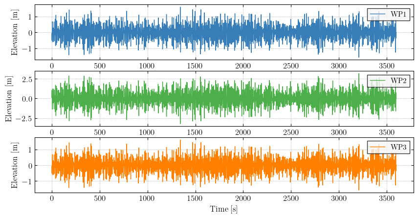
It appears that the elevation measured by WP2 is generally higher than that measured by the other two probes (WP1 and WP3).

Plot a zoomed-in view of the recorded surface elevation

For a more careful check of the time series, we plot a zoomed-in view of the recorded surface elevation for the three wave probes in a same plot.

linestyles = ["-", "-", "--"]
fig = plt.figure(figsize=(10, 2))
for i_plot in range(3):
    plt.plot(
        df_WP_seg["time"],
        df_WP_seg[f"WP{i_plot + 1}"],
        label=f"WP{i_plot + 1}",
        linestyle=linestyles[i_plot],
        color=colors[i_plot],
    )
plt.xlim(3000, 3100)
plt.xlabel("Time [s]")
plt.ylabel("Elevation [m]")
plt.legend()
print("Fig. 2: Zoomed-in wave elevation time series")
# fig.tight_layout()
plt.show()

Fig. 2: Zoomed-in wave elevation time series

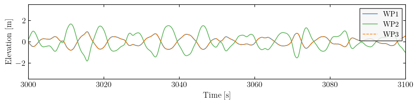
The signals from WP1 and WP3 seem to be nearly identical, while the signal from WP2 is out of phase.

Calculate basic statistics derived from a time-domain analysis

We compute the mean \(\mu\) and standard deviation \(\sigma\) of the three time series.

means_WP = df_WP_seg[["WP1", "WP2", "WP3"]].mean()
std_WP = df_WP_seg[["WP1", "WP2", "WP3"]].std()

stats_WP = pd.DataFrame({"Mean [m]": means_WP, "Std [m]": std_WP})
stats_WP.index.name = "Probe"
print(
    "Table 3: Statistics of wave elevation time series for the extracted time segment."
)
stats_WP

Table 3: Statistics of wave elevation time series for the extracted time segment.

	Mean [m]	Std [m]
Probe
WP1	-0.000139	0.461323
WP2	0.000278	0.922646
WP3	-0.000139	0.461323

The signals have a mean value under 1 millimeter. It can therefore be considered that they are zero-mean signals.

3. Compute a wave spectrum of measured surface elevation

Now, we would like to analyse the recorded surface elevation in the frequency domain. This includes the computation of a wave energy density spectrum, or wave spectrum, for each of the recorded signals.

To do this, we can use the scipy.signal.csd function from the Scipy package.

4. Extract the sea state parameters

5. Fit a standard wave spectra

In many engineering applications, such as the response analysis of marine structures exposed to waves, use of the wave spectrum is required in order to carry on the computations. In those cases, the sea state parameters can be exploited to reconstruct the wave spectrum by applying an adequately chosen parameterised spectrum.

There exist several standard forms of wave spectra. The choice of one form is application-specific and made based on the geographical area of study. Among other effects, the water depth, the predominance of wind sea over swell, or the opposite, and the fetch – defined as the length of the body of water that the wind blows over – should be considered (Mounet, 2023).

fmax = 0.5
Nf = 100
f = np.linspace(0, fmax, Nf)

References

1. Mounet, R.E.G. (2023). Sea State Estimation Based on Measurements from Multiple Observation Platforms. PhD Thesis. Technical University of Denmark. https://orbit.dtu.dk/en/publications/sea-state-estimation-based-on-measurements-from-multiple-observat