Last updated on Jun 04, 2026.

Example 3: Compute transfer functions for a simple geometry#

In this example application, it is shown how the linear wave-to-motion transfer functions (TRFs) can be estimated based on the basic information of the vessel’s main dimensions. The model assumes a simplified geometry of the vessel.

The following modules and packages are imported:

import matplotlib.pyplot as plt
import numpy as np

from netsse.dataset import load_example_data
from netsse.model.ship import heaveCF, pitchCF, rollCF
from netsse.tools.viz import fig_settings

===============================
Registration Request for NetSSE
To help us improve and better understand our user community, we kindly ask all users to register to use NetSSE. Registration is free.
If you have not already registered, please do so here:
https://forms.office.com/Pages/ResponsePage.aspx?id=I_FR8s7JjkSSdzS7KFkR2Xd1K-8FtOJFrL9QLVM8cJZUQ1hBS0VTN1E0OVU4QThTOTQ1WDA0TFg4Si4u
===============================

As can be seen in the above import, this example illustrates the use of the following NetSSE functions:

fig_settings(...),
load_example_data(...),
heaveCF(...), pitchCF(...), and rollCF(...) from the model.ship module.

1. Introduction#

Define default settings#

Those settings are used for the visual appearance of figures generated in this Python example.

fig_path, figcolors, props = fig_settings(font="serif", dpi=100, usetex=True)

Define the vessel’s main particulars#

These are the main dimensions of the vessel in study.

# Physical constants:
g = 9.80665  # Gravitational acceleration [m/s^2]

# Vessel parameters:
L = 232.02  # Length overall [m]
B = 39.60  # Beam [m]
D = 18.99  # Depth [m]
Td = 11.97  # Draught [m]
Delta = 95585  # Displacement [tons]
C_B = 0.848  # Block coefficient

2. Estimate the vessel’s RAOs of vertical motions via closed-form expressions#

In this section, the heave and pitch transfer functions of the vessel are estimated using semi-analytical closed-form expressions (CFEs) derived by Jensen et al. (2004) for a simplified vessel geometry. The expressions are implemented in NetSSE within the model.ship module.

Define the frequency vectors for the RAOs#

Those frequencies are defined as the (absolute) wave frequencies.

f0_CFE_max = 0.26  # Maximum frequency for the RAOs [Hz]
Nfreqs_CFE = 100  # Number of frequency points for the RAOs
f0_CFE = np.linspace(0.01, f0_CFE_max, Nfreqs_CFE)  # Frequency array for the RAOs [Hz]
om0_CFE = 2 * np.pi * f0_CFE  # Angular frequency array for the RAOs [rad/s]

Evaluate the closed-form expressions by Jensen et al. (2004) for the heave and pitch RAOs#

Let us assume head sea conditions, meaning that the waves are approaching the vessel from the bow, i.e., \(\beta = 180^\circ\). Moreover, the effect of forward speed is not considered, and zero forward speed is assumed.

beta = 180.0  # Relative wave heading [deg]
Vship = 0.0  # Vessel speed [m/s]

The expressions of the heave and pitch RAOs are evaluated. The pitch RAO is converted from radians to degrees.

hamp_CFE = np.squeeze(heaveCF(om0_CFE, beta, Vship, L, B, Td, C_B))
pamp_CFE = np.degrees(np.squeeze(pitchCF(om0_CFE, beta, Vship, L, B, Td, C_B)))

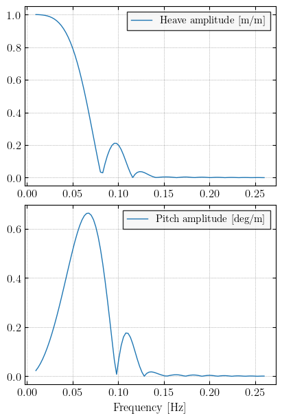
Plot the transfer functions estimated via the CFE#

fig, ax = plt.subplots(2, 1, figsize=(4, 6), constrained_layout=True)
ax[0].plot(f0_CFE, hamp_CFE, label=r"Heave amplitude [m/m]")
ax[1].plot(f0_CFE, pamp_CFE, label=r"Pitch amplitude [deg/m]")
for i in range(2):
    ax[i].grid()
    ax[i].legend()
ax[-1].set_xlabel(r"Frequency [Hz]")
print(
    "Fig. 1: CFE heave and pitch RAOs for a vessel at zero forward speed and head seas"
)
# fig.tight_layout()
plt.show()

Fig. 1: CFE heave and pitch RAOs for a vessel at zero forward speed and head seas

../_images/958919c3da349269227e1bf8f7094eaa7738fb457a23b6d9dd3f53bde732930d.png

3. Compare the estimates against strip theory results#

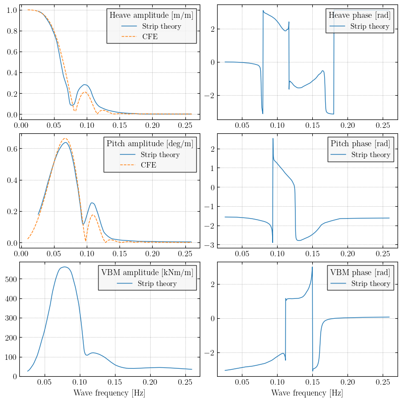
In this section, the RAO estimation results by the closed-form expressions (Jensen et al., 2004) are compared against reference RAOs obtained a linear strip theory solver, the so-called New Strip Method (Takagi and Ganno, 1967), in which the Lewis form approximation of ship cross-sections is adopted. For more detail, refer to Takami et al. (2026).

The amplitude and phase of the strip theory transfer functions of heave and pitch motions, as well as vertical bending moment (VBM), are provided here in a data file named "strip_theory_TRFs.txt".

Load the transfer functions derived by strip theory#

The data file is organized as shown in Table 1.

Table 1: File structure for the strip_theory_TRFs.txt data file.

	Column 0	Column 1	Column 2	Column 3	Column 4	Column 5	Column 6
Row 1	Frequency_1	Heave amp.	Heave phase	Pitch amp.	Pitch phase	VBM amp.	VBM phase
Row 2	Frequency_2
…	…	…	…	…	…	…	…
Row Nf	Frequency_Nf

ST_data = load_example_data("strip_theory_TRFs.txt", delimiter="\t")
f0_ST = ST_data[:, 0]
hamp_ST = ST_data[:, 1]
hphase_ST = ST_data[:, 2]
pamp_ST = ST_data[:, 3]
pphase_ST = ST_data[:, 4]
vamp_ST = ST_data[:, 5]
vphase_ST = ST_data[:, 6]

Plot the transfer functions estimated by strip theory#

The strip theory transfer functions are plotted together with the transfer functions estimated by the closed-form expressions (Jensen et al., 2004) for comparison.

legend_titles = [
    r"Heave amplitude [m/m]",
    r"Heave phase [rad]",
    r"Pitch amplitude [deg/m]",
    r"Pitch phase [rad]",
    r"VBM amplitude [kNm/m]",
    r"VBM phase [rad]",
]
fig, ax = plt.subplots(3, 2, figsize=(8, 8), constrained_layout=True)
ax[0, 0].plot(f0_ST, hamp_ST, label=r"Strip theory")
ax[0, 0].plot(f0_CFE, hamp_CFE, label=r"CFE", linestyle="--")
ax[0, 1].plot(f0_ST, hphase_ST, label=r"Strip theory")
ax[1, 0].plot(f0_ST, pamp_ST, label=r"Strip theory")
ax[1, 0].plot(f0_CFE, pamp_CFE, label=r"CFE", linestyle="--")
ax[1, 1].plot(f0_ST, pphase_ST, label=r"Strip theory")
ax[2, 0].plot(f0_ST, vamp_ST, label=r"Strip theory")
ax[2, 1].plot(f0_ST, vphase_ST, label=r"Strip theory")
for i in range(3):
    for j in range(2):
        ax[i, j].grid()
        ax[i, j].legend(title=legend_titles[i * 2 + j])
        ax[-1, j].set_xlabel(r"Wave frequency [Hz]")
print(
    "Fig. 2: Comparison of CFE and strip theory RAOs for heave, pitch, and vertical bending moment (VBM)"
)
# fig.tight_layout()
plt.show()

Fig. 2: Comparison of CFE and strip theory RAOs for heave, pitch, and vertical bending moment (VBM)

../_images/be97de8a5a308dfd1f9894e28e21b98ecb6b00a6e03d69f593aa14e375b47ee5.png

References#

Jensen, J.J., Mansour, A.E., & Olsen, A.S. (2004). Estimation of ship motions using closed-form expressions. Ocean Engineering 31(1), pp. 61–85. https://doi.org/10.1016/S0029-8018(03)00108-2.
Mounet, R.E.G. (2023). Sea State Estimation Based on Measurements from Multiple Observation Platforms. PhD Thesis. Technical University of Denmark. https://orbit.dtu.dk/en/publications/sea-state-estimation-based-on-measurements-from-multiple-observat.
Takagi, M. & Ganno, M. (1967). On the Accuracy of the Strip Theory, Used for a Calculation of Ship Motions in Waves. Journal of Zosen Kiokai 121, pp. 48–61. https://doi.org/10.2534/jjasnaoe1952.1967.48.
Takami, T., Nielsen, U.D., Mounet, R.E.G., Jensen, J.J., Mori, R. & Komoriyama, Y. (2026). Blind identification of incident waves and response transfer functions of a marine vessel based on measured responses. Expert Systems with Applications 296, 129236. https://doi.org/10.1016/j.eswa.2025.129236.